Analysis

Goals of this notebook

Important

This analysis is current through the Spring 2025 data release by the MLSPA.

We’ll explore MLS Salaries through history. We’ll start with the most recent data, then look back historically. A couple of questions that come to mind:

• Which players are getting paid the most this year?
• Which teams have the highest salary bill this year?
• How do team salary rankings compare over time?

Per the MLS Player’s Association, “compensation” is: The Annual Average Guaranteed Compensation (Guaranteed Comp) number includes a player’s base salary and all signing and guaranteed bonuses annualized over the term of the player’s contract, including option years.

Setup

library(tidyverse)
library(janitor)
library(scales)
library(ggrepel)
library(DT)

options(dplyr.summarise.inform = FALSE)
options(scipen = 999)

Import

Cleaned salary data

salaries <- read_rds("data-processed/mls-salaries.rds")

salaries |> glimpse()

Rows: 12,187
Columns: 9
$ year         <chr> "2007", "2007", "2007", "2007", "2007", "2007", "2007", "…
$ club_short   <chr> "CHI", "CHI", "CHI", "CHI", "CHI", "CHI", "CHI", "CHI", "…
$ last_name    <chr> "Armas", "Banner", "Barrett", "Blanco", "Brown", "Busch",…
$ first_name   <chr> "Chris", "Michael", "Chad", "Cuauhtemoc", "C.J.", "Jon", …
$ position     <chr> "M", "M", "F", "F", "D", "GK", "F", "D", "M", "D", "D", "…
$ base_salary  <dbl> 225000.0, 12900.0, 41212.5, 2492316.0, 106391.0, 58008.0,…
$ compensation <dbl> 225000.0, 12900.0, 48712.5, 2666778.0, 106391.0, 58008.0,…
$ club_long    <chr> "Chicago Fire FC", "Chicago Fire FC", "Chicago Fire FC", …
$ conference   <chr> "Eastern", "Eastern", "Eastern", "Eastern", "Eastern", "E…

Team colors data

You can see in MLS colors how I manually built these colors (and why).

# download.file("https://docs.google.com/spreadsheets/d/e/2PACX-1vQqXJxbbrBsikirZrGyXYV_G6cFZp_dYmcf52UfSYM7Kw3akGlkO5jKP8ZL8WtRA5qUJgFMNPG8JYov/pub?output=csv&&gid=1348329208", "data-processed/clubs-colors.csv")

mls_colors_data <- read_csv("data-processed/clubs-colors.csv")

Rows: 30 Columns: 7
── Column specification ────────────────────────────────────────────────────────
Delimiter: ","
chr (7): club_short, club_long, primary_color, secondary_color, tertiary_col...

ℹ Use `spec()` to retrieve the full column specification for this data.
ℹ Specify the column types or set `show_col_types = FALSE` to quiet this message.

mls_colors_data |> glimpse()

Rows: 30
Columns: 7
$ club_short      <chr> "ATL", "ATX", "CHI", "CIN", "CLB", "CLT", "COL", "DAL"…
$ club_long       <chr> "Atlanta United FC", "Austin FC", "Chicago Fire FC", "…
$ primary_color   <chr> "#80000a", "#00b140", "#FF0000", "#F05323", "#FEDD00",…
$ secondary_color <chr> "#221f1f", "#000000", "#141946", "#263B80", "#000000",…
$ tertiary_color  <chr> "#a19060", "#FFFFFF", "#7CCDEF", NA, NA, NA, "#D3D5D7"…
$ favored_color   <chr> "#80000a", "#00b140", "#7CCDEF", "#F05323", "#FEDD00",…
$ favored_nohex   <chr> "80000a", "00b140", "7CCDEF", "F05323", "FEDD00", "1A8…

Setting the most recent year of data

I’m creating an object called recent_year because at some point I’ll have new data and might want to just change the year.

recent_year <- "2025"

Players with highest salaries

Over all time

A searchable table of all players, all time.

sal_high <- salaries |> 
  arrange(compensation |> desc()) |> 
  select(!c(club_long, conference))

sal_high |> datatable()

Warning in instance$preRenderHook(instance): It seems your data is too big for
client-side DataTables. You may consider server-side processing:
https://rstudio.github.io/DT/server.html

Data takeaway: Messi money

Upon his signing on July 15, 2023, Lionel Messi became the highest paid player in the history of the MLS with a total compensation of $20.4 million. Lorenzo Insigne of Toronto was second at $15.5 million, the only other player earning more than $10 million within a year.

In most recent year

sal_high_recent <- salaries |> 
  filter(year == recent_year) |> 
  mutate(rank = min_rank(desc(compensation))) |> 
  relocate(rank) |> 
  arrange(compensation |> desc()) |> 
  select(!c(club_long, conference))

sal_high_recent

Teams with more than one player from top 10

sal_high_recent |> 
  filter(rank <= 10) |> 
  count(club_short, sort = T) |> 
  filter(n > 1)

Data takeaway: More than Messi

Inter Miami has three of the top 10 earners, while Toronto FC has two.

Difference with just base pay in 2025?

This looks at just the base salary as opposed to total compensation. No great changes at the top of the list.

sal_high_base <- salaries |> 
  arrange(base_salary |> desc()) |> 
  select(!c(club_long, conference, compensation))

sal_high_base |> filter(year == recent_year, base_salary >= 2000000) 

Hightest paid on Austin FC

Since we are in Austin, let’s see look at their 2025 roster spending.

sal_high_recent |> 
  filter(club_short == "ATX")

Owen Wolff has to be the best value on the team given he makes just over $220,000 and is a can’t-drop.

Team salaries

We’ll get per-year salaries by team, then look at just this year.

Highest team salaries over time

First get the total compensation for each team in each year.

sal_team <- salaries |> 
  group_by(year, club_long) |> 
  summarise(total_compensation = sum(compensation)) |> 
  arrange(total_compensation |> desc())

# peek at the top
sal_team |> filter(total_compensation > 20000000)

Then find the top team for each year.

top_sal_team_yr <- salaries |> 
  group_by(year, club_long) |> 
  summarise(total_compensation = sum(compensation)) |> 
  slice_max(total_compensation)

top_sal_team_yr

And note how often the teams have been the top spender.

top_sal_team_yr |> 
  ungroup() |> 
  tabyl(club_long) |> 
  adorn_totals("row") |>
  adorn_pct_formatting() |> 
  as_tibble()

Data takeaways: Toronto historically spends high

Looking at the most expensive rosters in the MLS of time, Toronto FC has seen of the top 10 highest entries. Over the past 17 years, Toronto has been the top spending team seven times, or 40% of the time. The L.A. Galaxy is next with five highest-spending years.

Highest salaries this year

And let’s look at this year.

sal_team_recent <- sal_team |> filter(year == recent_year)

# peek
sal_team_recent |> head(10)

Prep data for chart

Let’s round the numbers for our chart.

sal_team_recent_mil <- sal_team_recent |> 
  mutate(total_millions = (total_compensation / 1000000) |> round(1)) |> 
  left_join(
    mls_colors_data |> select(club_long, favored_color, favored_nohex),
    join_by(club_long)
  ) |>
  drop_na(favored_color)

sal_team_recent_mil

Let’s chart this

sal_team_recent_mil_plot <- sal_team_recent_mil |> 
  ggplot(aes(
    x = total_compensation,
    y = club_long |> reorder(total_compensation)
  )) +
  geom_col(fill = sal_team_recent_mil$favored_color) +
  scale_x_continuous(labels = label_dollar(scale_cut = cut_long_scale()),
                     limits = c(0,45000000)) +
  # geom_text(aes(label = paste("$", as.character(total_millions), sep = "")), color = "black", hjust = -.25) +
  labs(
    x = "Total team spending in $ millions",
    y = "",
    title = "Messi makes Miami top MLS spender",
    subtitle = str_wrap("Salaries includes each player's base salary plus all signing and guaranteed bonuses annualized over the term of the player's contract, including option years."),
    caption = "By: Christian McDonald. Source: Major League Soccer Players Association"
  ) +
  theme_minimal()

ggsave("figures/team-salary-recent.png", width = 7, height = 7)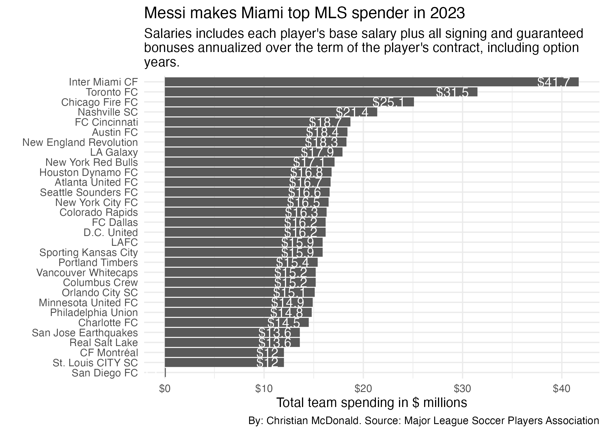

Warning: Removed 1 row containing missing values or values outside the scale range
(`geom_col()`).

One more look to see how many high-paid players on each team.

sal_high_recent |> 
  filter(compensation >= 5000000) |> 
  count(club_short, sort = T)

Data Takeaway: Miami, Toronto tops

Given the historic signing of Lionel Messi in 2023, it is no surprise that Inter Miami have the highest team salary for the 2024 season. Toronto ranks second on the power of having two players making over $5 million, Lorenzo Insigne and Federico Bernardeschi.

More than Messi

Which teams pay their entire team less than what the highest player makes?

top_player <- sal_high_recent |> 
  filter(!is.na(club_short)) |> 
  filter(rank == 1)

top_player_name <- 
  paste(top_player$first_name, top_player$last_name)

highest_comp <- top_player |> 
  pull(compensation)

more_than_top <- sal_high_recent |> 
  filter(!is.na(club_short)) |> 
  group_by(club_short) |> 
  summarise(total_comp = sum(compensation, na.rm = T)) |> 
  filter(total_comp < highest_comp)

more_than_top_nrow <- more_than_top |> nrow()

In 2025 the highest paid player was Lionel Messi making $20,446,667. There are 21 teams that pay less than that for their entire roster.

Team spending over time

Let’s look at team spending over the past five years. To do this, we have to create a ranking for the spending.

• I’m removing players not affiliated with teams
• When I added a third column to the group because I wanted to use long names for something, the ranking broke. I had to break the group then use the .by argument for rank().

sal_team_rank <- salaries |> 
  filter(club_short != "MLS" | club_short |> is.na()) |> 
  group_by(year, club_short, club_long) |> 
  summarise(
    total_comp = sum(compensation, na.rm = TRUE)
  ) |> 
  arrange(year, total_comp |> desc()) |> 
1  ungroup() |>
2  mutate(rank = rank(-total_comp), .by = year)

# peek
sal_team_rank |> head(20)

1

I break the group_by here.

2

Then I set the ranking to work by year.

Visualizing all of them would be tricky. Let’s do the top five over last five years.

sal_team_rank_top <- sal_team_rank |> 
  filter(rank <= 5,
         year >= (as.numeric(recent_year) - 4)) |> 
  left_join(mls_colors_data |> select(club_short, favored_color, favored_nohex), join_by(club_short))

sal_team_rank_top |> 
  filter(club_short == "MIA")

Peek at this a different way

sal_team_rank_top |> 
  select(-total_comp) |> 
  pivot_wider(names_from = year, values_from = rank)

Let’s visualze spending rank

We are using

sal_team_rank_top_plot <- sal_team_rank_top |> 
  ggplot(aes(x=year, y=rank, color = favored_color, group = club_short)) +
  geom_point(size = 3) +
  geom_line() +
  scale_y_reverse() +
  scale_color_identity(aes(color = favored_color)) +
  geom_label_repel(aes(label = club_short), color = "black", size = 3) +
  labs(
    title = "Miami's spending was increasing before Messi",
subtitle = str_wrap("Maimi and the L.A. Galaxy are the only MLS teams to rank as a top five spender in each of the past five years. Miami's spending rank was climbing before Lionel Messi joined in 2023."),
    color = "Club",
    x = NULL,
    y = "Spending Rank",
    caption = "By: Christian McDonald. Source: Major League Soccer Players Association"
  ) +
  theme_minimal()


ggsave("figures/sal_team_rank.png")

Saving 7 x 5 in image

Let’s count how many times each team is in this list.

sal_team_rank_top |> 
  count(club_long, sort = T)

Data Takeaway: Miami and LA

Both Miami and the LA Galaxy have been among the top spending teams over the past five years. Toronto FC have been top spenders in four of the last five years.